Running a likelihood profile on a FIMS model

library(FIMSdiags)
library(FIMS)
packageVersion("FIMS")
#> [1] '0.7.1'

clear()

Set up FIMS model

Following the minimal FIMS demo vignette, we will set up a FIMS model and run it. We need to run it initially to get the MLE parameter estimates. For this example we are using the dataset included in the FIMS package and creating a set of default parameters.

# Load sample data
data("data1")
# Prepare data for FIMS model
data_4_model <- FIMSFrame(data1)

# Create parameters
parameters <- data_4_model |>
  create_default_configurations() |>
  create_default_parameters(data = data_4_model)

# Run the  model with optimization
base_model <- parameters |>
  initialize_fims(data = data_4_model) |>
  fit_fims(optimize = TRUE)
#> ✔ Starting optimization ...
#> ℹ Restarting optimizer 3 times to improve gradient.
#> ℹ Maximum gradient went from 0.02469 to 0.00037 after 3 steps.
#> ✔ Finished optimization
#> ✔ Finished sdreport
#> ℹ FIMS model version: 0.7.1
#> ℹ Total run time was 10.18995 seconds
#> ℹ Number of parameters: fixed_effects=77, random_effects=0, and total=77
#> ℹ Maximum gradient= 0.00037
#> ℹ Negative log likelihood (NLL):
#> • Marginal NLL= 3240.1261
#> • Total NLL= 3240.1261
#> ℹ Terminal SB= 1803.27712

# Clear memory post-run
clear()

Run likelihood profile

Once we have a model that is fit, we can run a likelihood profile analysis to see the impact of each data type on a given parameter. In this example, we will test the impact on R₀ but any value can be tested by changing the parameter_name argument. Note: The parameter name must match what it is called in the label column of the parameters tibble. An optional input is the module_name the parameter is associated with. However, as long as there is only one parameter with that name, module_name can be left NULL. The run_fims_likelihood function takes a fitted FIMS model, finds the MLE estimate for the parameter being profiled over (in this case R₀), and profiles over a vector of values based on the min, max, and length the user inputs. In the example below, it will profile over 5 values that range from the MLE value - 1 to the MLE value + 1. If you are running many models at once, it can be computationally more efficient to use multiple cores. To do this, change the n_cores argument to as many as you want/can use. NOTE: If left empty, the default for n_cores is one less than the number of cores on your machine so this could unexpectedly use up a lot of your computing power.

like_fit <- run_fims_likelihood(
  model = base_model,
  parameters = parameters,
  parameter_name = "log_rzero", 
  data = data1,
  n_cores = 1,
  min = -1,
  max = 1,
  length = 5
)

Visualize results

To visualize the profile, use the function plot_likelihood. The plot shows the change in total likelihood over the R₀ values profiled in the solid black line, and the change in likelihood for each data type in the color lines below it. This plot indicates that the R₀ value estimated by the base model (13.9) is the value that leads to the lowest likelihood and all of the data types support this (i.e. the data do not conflict).

plot_likelihood(like_fit)
#> Scale for colour is already present.
#> Adding another scale for colour, which will replace the existing scale.
#> Saving 9 x 7 in image

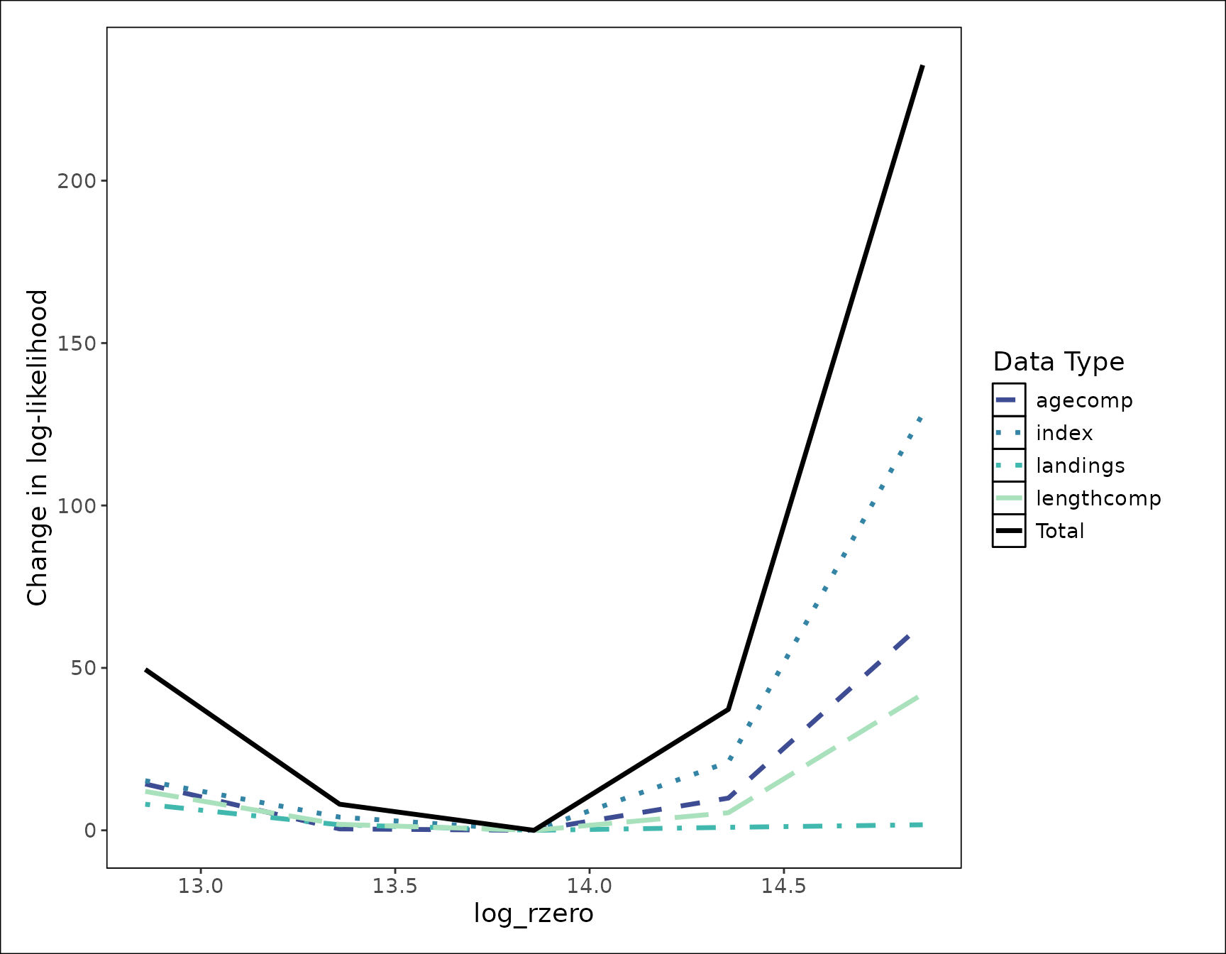
This function creates a ggplot object that can be customized and added onto as a normal ggplot can. The default theme is stockplotr::theme_noaa, however to change the theme or colors used, you can simply add them after the main plot function.

plot_likelihood(like_fit) +
ggplot2::theme_bw()
#> Scale for colour is already present.
#> Adding another scale for colour, which will replace the existing scale.
#> Saving 9 x 7 in image

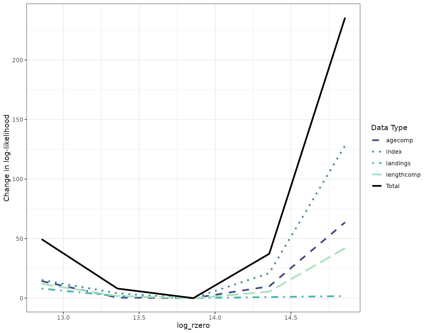
Clean up

Once you have finished running a FIMS model, it is always good practice to clear the C++ memory from one FIMS model run to the next.

clear()