Meta-analyses with the fishprior R package • fishprior

The vignette provides a slightly more complicated example of how to use the fishprior package to combine parameters into a meta-analysis. The summarize_fishbase_traits() function produces summary statistics across studies, weighting estimates equally and ignoring sample sizes or standard errors of estimates. We provide two case studies below, first examining maximum length of European mackerel (weighting studies by sample size), and second examining growth rates of sablefish (weighting studies by standard errors).

FishBase includes sample sizes (Number) and standard errors (SE) when available, however these may not be available for most records, and there may be variability in reporting by species or trait type. For full details, see the following tables

FishBase.tables.used
rfishbase::popgrowth
rfishbase::popchar
rfishbase::poplw
rfishbase::maturity
rfishbase::fecundity

Combining estimates using sample sizes

To illustrate how point estimates may combined in a more traditional meta-analysis, we’ll use data from the European mackerel (Scomber scombrus). Data can be obtained from FishBase using get_fishbase_traits() – more detailed information is in the introductory vignette. We will focus this example on maximum length (LengthMax) because it is one of the variables in rfishbase::poplw() that has an associated sample size, but not standard error.

species_list <- c(
  "Scomber scombrus"
)
example_base_raw <- get_fishbase_traits(spec_names = species_list)
example_base_raw

## # A tibble: 288 × 22
##    rfishbase SpecCode Sex     PopGrowthRef DataSourceRef Locality      YearStart
##    <chr>        <int> <chr>          <int>         <int> <chr>             <int>
##  1 popgrowth      118 unsexed          207            NA Northwest At…        NA
##  2 popgrowth      118 unsexed          207            NA Northwest At…        NA
##  3 popgrowth      118 unsexed          207            NA Northwest At…        NA
##  4 popgrowth      118 unsexed          207            NA Northwest At…        NA
##  5 popgrowth      118 unsexed          207            NA Northwest At…        NA
##  6 popgrowth      118 unsexed          312          1208 ICNAF Subare…      1974
##  7 popgrowth      118 unsexed          312          1208 ICNAF Subare…      1974
##  8 popgrowth      118 unsexed          312          1208 ICNAF Subare…      1974
##  9 popgrowth      118 unsexed          312          1208 ICNAF Subare…      1974
## 10 popgrowth      118 unsexed          312          1207 New England        1973
## # ℹ 278 more rows
## # ℹ 15 more variables: YearEnd <int>, Number <dbl>, Type <chr>, C_Code <chr>,
## #   E_CODE <dbl>, SourceRef <int>, StockCode <dbl>, AgeMatRef <int>,
## #   trait <chr>, value <dbl>, SE <dbl>, SD <dbl>, country <chr>,
## #   EcosystemName <chr>, Species <chr>

There are differences in reporting between Number and SE, with fewer studies having standard errors reported. There may be some rounding or reporting issues with SE, because at least one of the values is 0. There’s quite a bit of variation by trait type, with estimates from studies estimating length-weight regressions reporting Number more commonly than other studies,

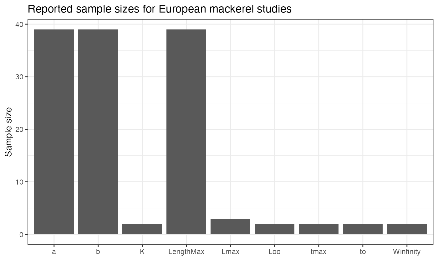
We will filter out studies that don’t report Number, but an alternative approach would be to set the Number for these studies to some small value (the smallest reported across all studies, or 1, etc)

filtered_traits <- dplyr::filter(
  example_base_raw,
  Number > 0,
  trait %in% c("LengthMax")
)

Variance weighting

The first way to combine estimates is by applying variance weighting. To do this, we use Number as the weights for the weighted mean and variance,

weighted_summary <- filtered_traits |>
  dplyr::summarise(
    weighted_mean = weighted.mean(value, w = Number),
    simple_mean = mean(value),
    weighted_var = sum(Number * (value - weighted_mean)^2) / sum(Number),
    weighted_se = sqrt(weighted_var / dplyr::n()),
    total_n = sum(Number),
    n_studies = dplyr::n()
  )
weighted_summary

## # A tibble: 1 × 6
##   weighted_mean simple_mean weighted_var weighted_se total_n n_studies
##           <dbl>       <dbl>        <dbl>       <dbl>   <dbl>     <int>
## 1          45.0        41.6         5.28       0.368   61367        39

The vertical blue lines here represent the weighted mean (and 95% confidence intervals); the weighted mean is slightly larger than the simple mean (42).

## `stat_bin()` using `bins = 30`. Pick better value `binwidth`.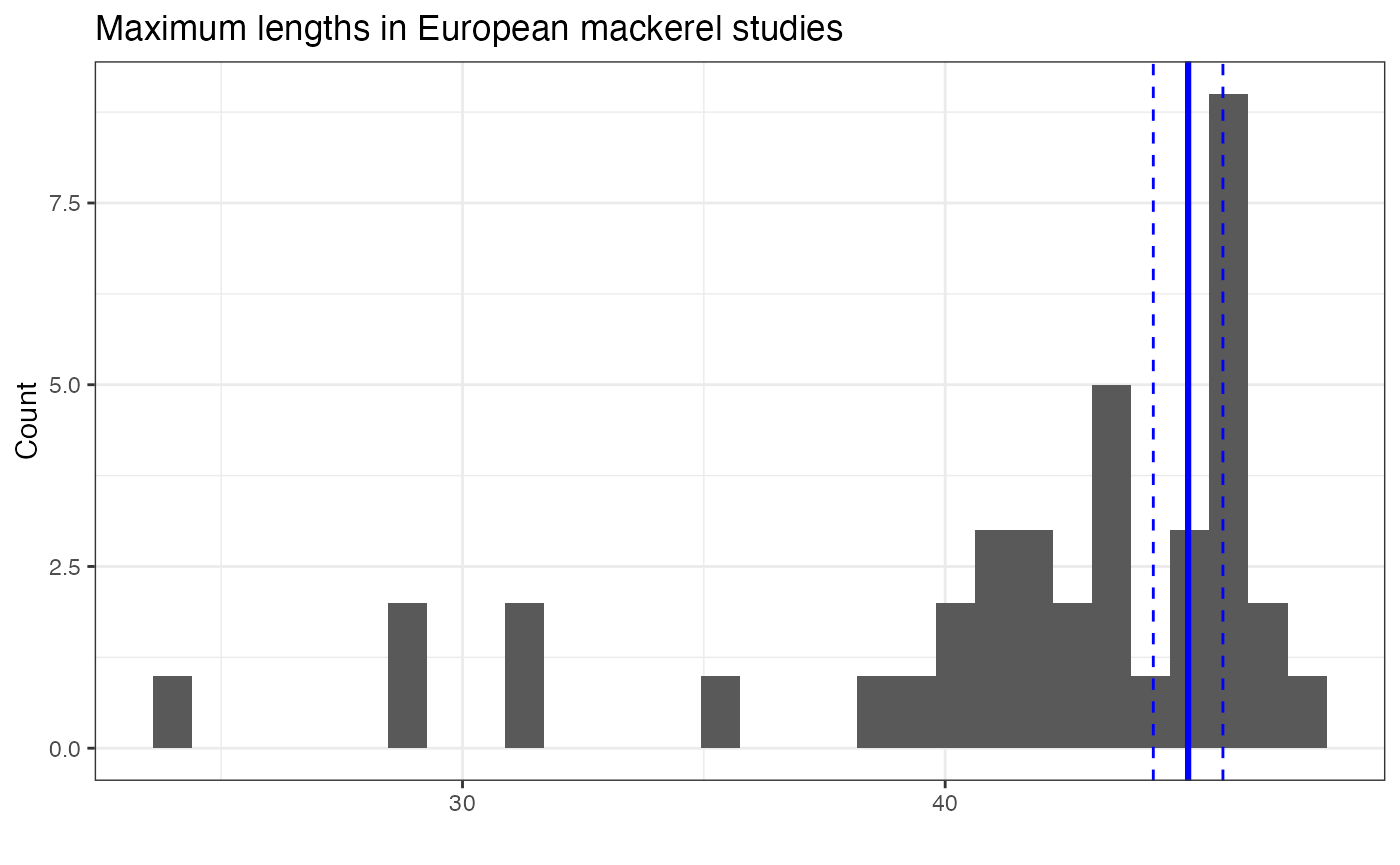

Model based weighting

Without the reported study specific standard errors, it is difficult to do a true meta-analysis. However we can estimate a common mean and observation variance, which is another way to use the sample sizes as weights. The reported mean length $y_i$ can be assumed to be an observation of the true study-specific unobserved mean length $\theta_i$ , where $\sigma$ represents the variance across studies,

$y_i \sim Normal(\theta_i, \frac{\sigma}{\sqrt{n_i}})$ and then the random effects can be estimated with a common hyperparameters

$\theta_i \sim Normal(\mu, \tau)$

To fit this model in brms, we can use the following code. Because maximum size can be skewed, we’ll fit the model in log space,

library(brms)
filtered_traits$sqrt_n <- 1 / sqrt(filtered_traits$Number)
filtered_traits$study_id <- seq_len(nrow(filtered_traits))
filtered_traits$log_n <- log(filtered_traits$value)

formula <- bf(
  log_n ~ 1,
  sigma ~ 0 + sqrt_n
)

fit <- brm(
  formula,
  data = filtered_traits,
  family = gaussian(),
  chains = 4,
  iter = 5000,
  control = list(adapt_delta = 0.999)
)

Combining estimates using meta-analysis

For cases where the standard errors exist, a second approach is to do a true meta-analysis and use the standard errors as weights. For this example, we’ll focus a meta-analysis on the growth coefficient (k) of sablefish (Anoplopoma fimbria)

species_list <- c(
  "Anoplopoma fimbria"
)
sablefish_traits <- get_fishbase_traits(spec_names = species_list)

filtered_traits <- dplyr::filter(
  sablefish_traits,
  SE > 0,
  trait %in% c("K")
)

There’s a small number of studies here from 2 regions in the Pacific Ocean, and if we look at breakdown by region, there seems to be substantially smaller values in Alaska.

Locality	value	SE
West coast	0.499	0.047
West coast	0.481	0.083
Gulf of Alaska	0.117	0.024
Gulf of Alaska	0.106	0.008
West coast	0.472	0.055
West coast	0.556	0.108
Gulf of Alaska	0.120	0.140
Gulf of Alaska	0.126	0.044

It probably makes more sense for interpretation and estimation to focus on a single region, so we will only use estimates from Alaska

ak_traits <- dplyr::filter(
  filtered_traits,
  Locality %in% c("Gulf of Alaska")
)

We consider three meta-analytic models of increasing complexity, each building on the previous by relaxing assumptions about the sources of variance in the data.

Model 1: Known standard errors only

The simplest meta-analytic model treats the reported standard errors as fully characterizing observation-level uncertainty, with no additional residual variance:

$y_i \sim Normal(\mu, \text{SE}_i)$

where $y_i$ is the observed trait value for study $i$ , $\mu$ is the pooled mean (the single parameter being estimated), and $\text{SE}_i$ is the known standard error from FishBase, treated as fixed. This is the classical fixed-effects meta-analytic assumption — the SE accounts for all variance and there is no additional unexplained noise.

fit1 <- brm(
  value | se(SE) ~ 1,
  data = ak_traits,
  prior = prior(normal(0, 10), class = Intercept),
  chains = 4, iter = 2000,
  control = list(adapt_delta = 0.999)
)

Model 2: Known standard errors with residual variance

In practice, the reported SE may not capture all sources of variation. Model 2 relaxes the assumption that SE fully characterizes observation uncertainty by additionally estimating a residual variance $\sigma$ :

$y_i \sim Normal(\mu, \sqrt{\text{SE}_i^2 + \sigma^2})$

This model has 2 parameters being estimated, $\mu$ and $\sigma$ ). This is specified in brms using sigma = TRUE within the se() function:

fit2 <- brm(
  value | se(SE, sigma = TRUE) ~ 1,
  data = ak_traits,
  prior = c(
    prior(normal(0, 10), class = Intercept),
    prior(exponential(1), class = sigma)
  ),
  chains = 4, iter = 2000,
  control = list(adapt_delta = 0.999)
)

Model 3: Known standard errors with residual variance and random effects

Model 3 is the most general formulation, adding a study-level random effect $\delta_i$ to capture among-study variation beyond what is explained by the known SE and residual variance:

$y_i \sim Normal(\mu + \delta_i, \sqrt{\text{SE}_i^2 + \sigma^2})$ $\delta_i \sim Normal(0, \tau)$

where $\tau$ is the standard deviation of study-level random effects, representing among-study heterogeneity. This is the most flexible model but also has the most parameters estimated — with only a small number of studies, $\tau$ and $\sigma$ may be difficult to distinguish and estimates may be sensitive to priors.

fit3 <- brm(
  value | se(SE, sigma = TRUE) ~ 1 + (1 | study),
  data = ak_traits,
  prior = c(
    prior(normal(0, 10), class = Intercept),
    prior(exponential(1), class = sigma),
    prior(exponential(1), class = sd)
  ),
  chains = 4, iter = 2000,
  control = list(adapt_delta = 0.999)
)