Simple projections using FIMS • FIMS

Projections in FIMS

Projections in FIMS can occur during the model-fitting process. That is, you can extend your time series as many years into the future that you wish with fixed values of catch or fixed fishing mortality values to project the population forward in time while estimating parameters. This dual process during the estimation phase allows you to set priors on future values and integrate estimated uncertainty into the projection period.

As we work to set up various inputs and outputs for necessary management quantities for each region, we encourage you to join the FIMS Discussion Board to voice your thoughts about quantities that should be included. Second, please report bugs in the code to our Issues page.

library(FIMS)
library(ggplot2)
library(stockplotr)

# Use the {stockplotr} theme for all figures
# ggplot2::theme_set(stockplotr::theme_noaa())

# clear memory
clear()

Without projections

The code below uses the built-in data within FIMS and sets up a simple catch-at-age configuration object that will work with the data. These data and configuration objects will be used for to create an extended data set in the next section. More details about the chunk below can be found in the introductory vignette.

# Bring the package data into your environment
data("data_big")
# Prepare the package data for being used in a FIMS model
data_4_model <- FIMSFrame(data_big)

# Create default model configurations based on the data
default_configurations <- create_default_configurations(data = data_4_model)

Projections

Here we specify how many years beyond the terminal data year that projections extend out. This could be short (<10) for constant catch scenarios or long (one or more generations) to calculate equilibrium reference points such as fishing mortality at maximum sustainable yield or biomass at maximum sustainable yield.

years_of_projection <- 10

Data

Below, we show how you can update your data to include 10 years of projections by extending the terminal year. Second, FIMS::FIMSFrame() will fill in missing years of data for each data type based on your new maximum year in your data. These missing years use a value of -999 for each data type but users must provide the uncertainty level associated with the missing data because by default it will be filled with NA.

In the future, we will integrate more of the process below coded below into wrapper functions but as of FIMS version 0.8.0 some manipulation of the data is needed.

# Add a single row of landings to the original data for the maximum year you
# want to project to
data_big_with_extra_year <- dplyr::add_row(
  data_big,
  type = "landings",
  timing = get_end_year(data_4_model) + years_of_projection,
  name = "fleet1",
  value = -999,
  unit = "mt"
) |>
  dplyr::filter(
    !(type == "age_to_length_conversion" | type == "length_comp")
  )
data_4_projections <- data_big_with_extra_year |>
  # Add on weight_at_age because you don't want these filled with -999
  dplyr::bind_rows(
    dplyr::filter(
      data_big,
      type == "weight_at_age",
      timing == 1
    ) |>
      dplyr::select(-timing) |>
      merge(
        data.frame(timing = max(data_big[["timing"]], na.rm = TRUE):(max(data_big[["timing"]], na.rm = TRUE) + years_of_projection))
      )
  ) |>
  # Make a FIMSFrame object out of this data frame with the extra row to add all
  # of the other missing years for each data type
  FIMSFrame() |>
  # Extract the data object
  get_data() |>
  # Change the uncertainty values for each data type these values will
  # propagate forward into the log standard deviation values in the model
  # specifications
  dplyr::mutate(
    uncertainty = ifelse(
      type %in% c("landings") & value == -999,
      0.00999975,
      uncertainty
    ),
    uncertainty = ifelse(
      type %in% c("index") & value == -999,
      0.19804220,
      uncertainty
    ),
    uncertainty = ifelse(
      type %in% c("age_comp", "length_comp") & value == -999,
      0,
      uncertainty
    )
  ) |>
  # Make a FIMSFrame out of the altered data frame
  FIMSFrame()

Model

The default configuration from a model without projections can be used as the default configuration. After the parameter configuration is created it must be manipulated to alter the default parameters for things like selectivity, fishing mortality, etc. We believe that it is easier to alter default configurations rather than creating your own from scratch. So, much of what is done below for projections was also done in the introductory vignette.

The major difference below compared to a model without projections is that the recruitment deviations for the projection period are fixed at zero. Because the new data object has all years, FIMS::create_default_parameters() will ensure that all time-series parameters, e.g., natural mortality, have the correct dimensions.

# Take the default configuration with the new data to create some default
# parameters that we alter to make the model behave a little better
parameters_projection <- create_default_parameters(
  configurations = default_configurations,
  data = data_4_projections
) |>
  tidyr::unnest(cols = data) |>
  # Update log_Fmort initial values for Fleet1
  # Project the population forward with the terminal year mortality values.
  # More advanced approaches are included in
  # tests/testthat/test-projections-looped.R
  dplyr::rows_update(
    tibble::tibble(
      fleet_name = "fleet1",
      label = "log_Fmort",
      time = get_start_year(data_4_projections):
      get_end_year(data_4_projections),
      value = log(c(
        0.009459165, 0.027288858, 0.045063639,
        0.061017825, 0.048600752, 0.087420554,
        0.088447204, 0.186607929, 0.109008958,
        0.132704335, 0.150615473, 0.161242955,
        0.116640187, 0.169346119, 0.180191913,
        0.161240483, 0.314573212, 0.257247574,
        0.254887252, 0.251462108, 0.349101406,
        0.254107720, 0.418478117, 0.345721184,
        0.343685540, 0.314171227, 0.308026829,
        0.431745298, 0.328030899, 0.499675368,
        rep(0.499675368, years_of_projection)
      ))
    ),
    by = c("fleet_name", "label", "time")
  ) |>
  # Fix the projection period log_Fmort to constant
  dplyr::rows_update(
    tibble::tibble(
      label = "log_Fmort",
      time = (get_end_year(data_4_projections) - years_of_projection + 1):
      get_end_year(data_4_projections),
      estimation_type = rep("constant", years_of_projection)
    ),
    by = c("label", "time")
  ) |>
  # Update selectivity parameters and log_q for survey1
  dplyr::rows_update(
    tibble::tibble(
      fleet_name = "survey1",
      label = c("inflection_point", "slope", "log_q"),
      value = c(1.5, 2, log(3.315143e-07))
    ),
    by = c("fleet_name", "label")
  ) |>
  # Update log_devs in the Recruitment module (time steps 2-end)
  dplyr::rows_update(
    tibble::tibble(
      label = "log_devs",
      time = (get_start_year(data_4_projections) + 1):
      get_end_year(data_4_projections),
      value = c(
        0.43787763, -0.13299042, -0.43251973, 0.64861200, 0.50640852,
        -0.06958319, 0.30246260, -0.08257384, 0.20740372, 0.15289604,
        -0.21709207, -0.13320626, 0.11225374, -0.10650836, 0.26877132,
        0.24094126, -0.54480751, -0.23680557, -0.58483386, 0.30122785,
        0.21930545, -0.22281699, -0.51358369, 0.15740234, -0.53988240,
        -0.19556523, 0.20094360, 0.37248740, -0.07163145,
        # recruitment deviations are fixed at zero for the projections
        rep(0, years_of_projection)
      ),
      estimation_type = "random_effects"
    ),
    by = c("label", "time")
  ) |>
  # Fix the projection log recruitment deviations at zero
  dplyr::rows_update(
    tibble::tibble(
      label = "log_devs",
      time = (get_end_year(data_4_projections) - years_of_projection + 1):
      get_end_year(data_4_projections),
      estimation_type = rep("constant", years_of_projection),
      distribution_type = rep(NA, years_of_projection),
      distribution = rep(NA, years_of_projection)
    ),
    by = c("label", "time")
  ) |>
  # Update log_sd for log_devs in the Recruitment module
  dplyr::rows_update(
    tibble::tibble(
      module_name = "Recruitment",
      label = "log_sd",
      value = 0.4,
      estimation_type = "fixed_effects"
    ),
    by = c("module_name", "label")
  ) |>
  # Update inflection point and slope parameters in the Maturity module
  dplyr::rows_update(
    tibble::tibble(
      module_name = "Maturity",
      label = c("inflection_point", "slope"),
      value = c(2.25, 3)
    ),
    by = c("module_name", "label")
  ) |>
  # Update log_init_naa values in the Population module
  dplyr::rows_update(
    tibble::tibble(
      label = "log_init_naa",
      age = 1:get_n_ages(data_4_projections),
      value = c(
        13.80944, 13.60690, 13.40217, 13.19525, 12.98692, 12.77791,
        12.56862, 12.35922, 12.14979, 11.94034, 11.73088, 13.18755
      )
    ),
    by = c("label", "age")
  )

Reference-point targets are currently achieved by specifying a prior on spawning_biomass_ratio, a derived population quantity, in the final year/s of the projection period. Additionally, a prior can be specified on log_f_multiplier, which is a simple annual multiplier of fishing mortality, i.e., F_mort that allows the total fishing mortality for the population to be adjusted while keeping relative fleet effort constant by fixing log_Fmort. This approach allows the annual log_f_multiplier to be estimated while ensuring that total fishing mortality is held constant during the projection period and achieves the spawning biomass target.

The wrapper functions used in this vignette are not yet capable of setting up priors so the full projection approach is not included here. This is a high-priority development goal that is in progress. Examples of setting up constraints on log_f_multiplier and a prior on spawning_biomass_ratio can be found in the test-projections-looped.R test files used to verify this approach.

Model fit

Regardless if there are projections or not, the model is fit using the FIMS::fit_fims(), which facilitates that the model output will be in the same format that users are used to.

projection_fit <- parameters_projection |>
  initialize_fims(data = data_4_projections) |>
  fit_fims(optimize = TRUE)

## ✔ Starting optimization ...
## ℹ Restarting optimizer 3 times to improve gradient.
## ℹ Maximum gradient went from 0.00316 to 0.00022 after 3 steps.
## ✔ Finished optimization
## ✔ Finished sdreport
## ℹ FIMS model version: 0.9.2
## ℹ Total run time was 1.27309 minutes
## ℹ Number of parameters: fixed_effects=49, random_effects=29, and total=78
## ℹ Maximum gradient= 0.00022
## ℹ Negative log likelihood (NLL):
## • Marginal NLL= 1624.68892
## • Total NLL= 1560.83065
## ℹ Terminal SB= 993.45041

clear()

Model summaries

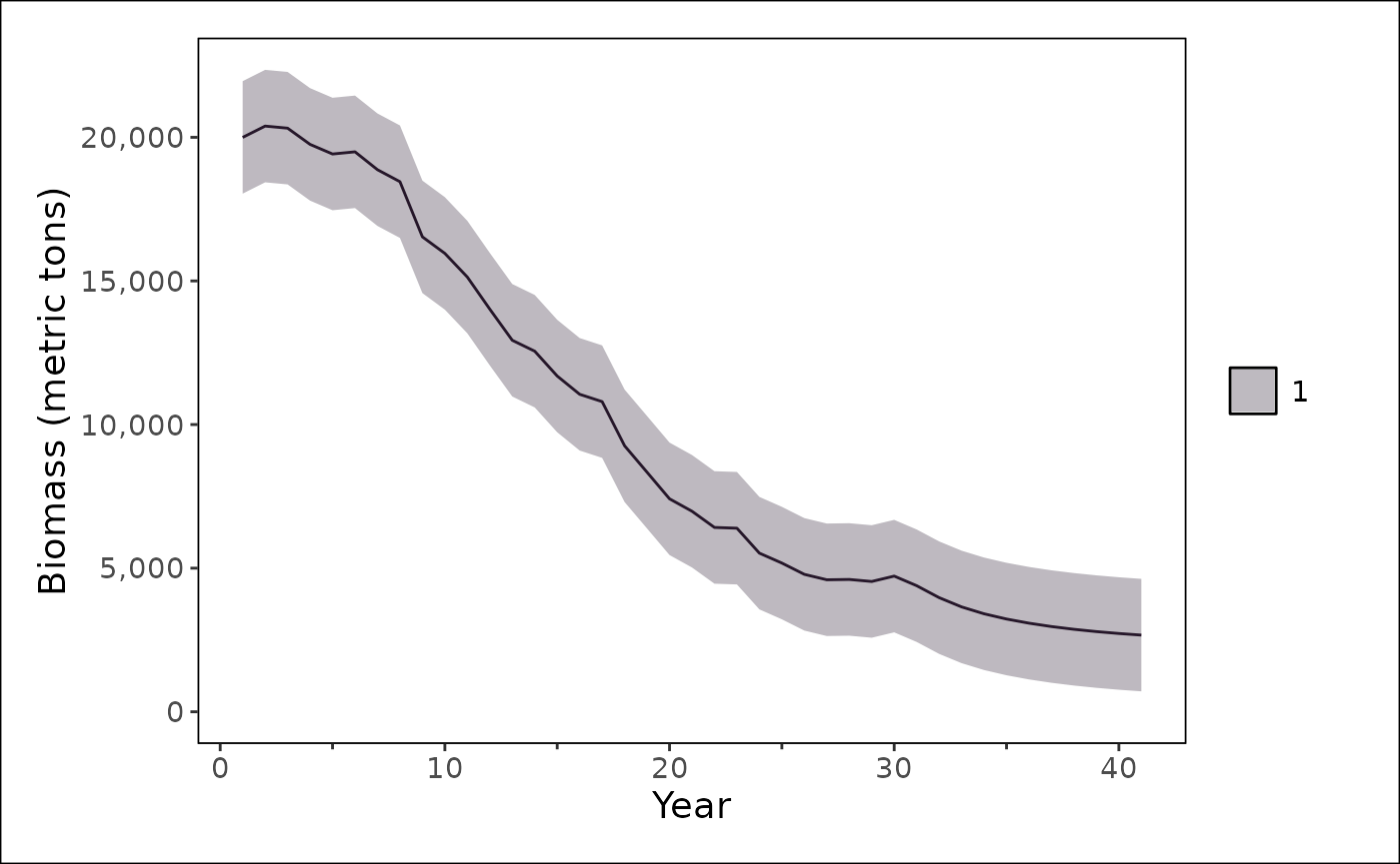
We use {stockplotr} to plot the model results. In the code below, we pass a single model to stockplotr::plot_biomass() but the list can contain multiple models, where the start and end year of each model that is included need not align. Thus, if we had fit the model without projections we could have plotted that here as well for comparison.

stockplotr::plot_biomass(
  list(
    "age" = get_estimates(projection_fit) |>
      dplyr::mutate(
        uncertainty_label = "se",
        year = year_i,
        estimate = estimated
      )
  )
)

## Warning: Unknown or uninitialised column: `era`.

## Warning in max(dat$year[dat$era == era_name], na.rm = TRUE): no non-missing
## arguments to max; returning -Inf

## Warning: Removed 1 row containing missing values or values outside the scale range
## (`geom_hline()`).

## Warning: Removed 1 row containing missing values or values outside the scale range
## (`geom_text()`).

Plot of spawning biomass for projection model.