Running diagnostics on a FIMS model • FIMS

library(FIMS)
packageVersion("FIMS")
#> [1] '0.9.3.9000'
clear()

Set up FIMS model

Following the minimal FIMS demo vignette, we will set up a FIMS model and run it. This model will contain the all years of data and will be our reference model (see section below for more information about reference models). We need to run it initially to get the MLE parameter estimates. For this example we are using the dataset included in the FIMS package and creating a set of default parameters.

# Load sample data
data("data_big")
# Prepare data for FIMS model
data_4_model <- FIMSFrame(data_big)

# Create parameters
parameters <- data_4_model |>
  create_default_configurations() |>
  create_default_parameters(data = data_4_model)

# Run the  model with optimization
base_model <- parameters |>
  initialize_fims(data = data_4_model) |>
  fit_fims(optimize = TRUE)
#> ✔ Starting optimization ...
#> ℹ Restarting optimizer 3 times to improve gradient.
#> ℹ Maximum gradient went from 0.00165 to 0.00031 after 3 steps.
#> ✔ Finished optimization
#> ✔ Finished sdreport
#> ℹ FIMS model version: 0.9.3.9000
#> ℹ Total run time was 1.43587 minutes
#> ℹ Number of parameters: fixed_effects=49, random_effects=29, and total=78
#> ℹ Maximum gradient= 0.00031
#> ℹ Negative log likelihood (NLL):
#> • Marginal NLL= 3231.28735
#> • Total NLL= 3164.86339
#> ℹ Terminal SB= 1728.68508

# Clear memory post-run
clear()

Likelihood profile

Once we have a model that is fit, we can run a likelihood profile to see the impact of each data type on a given parameter. In this example, we will test the impact on R₀ but any value can be tested by changing the parameter_name argument. Note: The parameter name must match what it is called in the label column of the parameters tibble. An optional input is the module_name the parameter is associated with. However, as long as there is only one parameter with that name, module_name can be left NULL. run_fims_likelihood() function takes a fitted FIMS model, finds the MLE estimate for the parameter being profiled over (in this case R₀), and profiles over a vector of values based on the min, max, and length user inputs. In the example below, it will profile over 5 values that range from the MLE value - 1 to the MLE value + 1. If you are running many models at once, it can be computationally more efficient to use multiple cores. To do this, change the n_cores argument to as many as you want/can use. NOTE: If left empty, the default for n_cores is one less than the number of cores on your machine so this could unexpectedly use up a lot of your computing power.

like_fit <- run_fims_likelihood(
  model = base_model,
  parameters = parameters,
  parameter_name = "log_rzero",
  data = data_big,
  n_cores = 3,
  min = -1,
  max = 1,
  length = 3
)

Visualize results

Use plot_likelihood() to visualize the profile. The plot shows the change in total likelihood over the R₀ values profiled in the solid black line and the change in likelihood for each data type in the color lines below it. This plot indicates that the R₀ value estimated by the base model (13.9) is the value that leads to the lowest likelihood and all of the data types support this (i.e., the data do not conflict).

fig_likelihood_profile <- plot_likelihood(like_fit)
print(fig_likelihood_profile)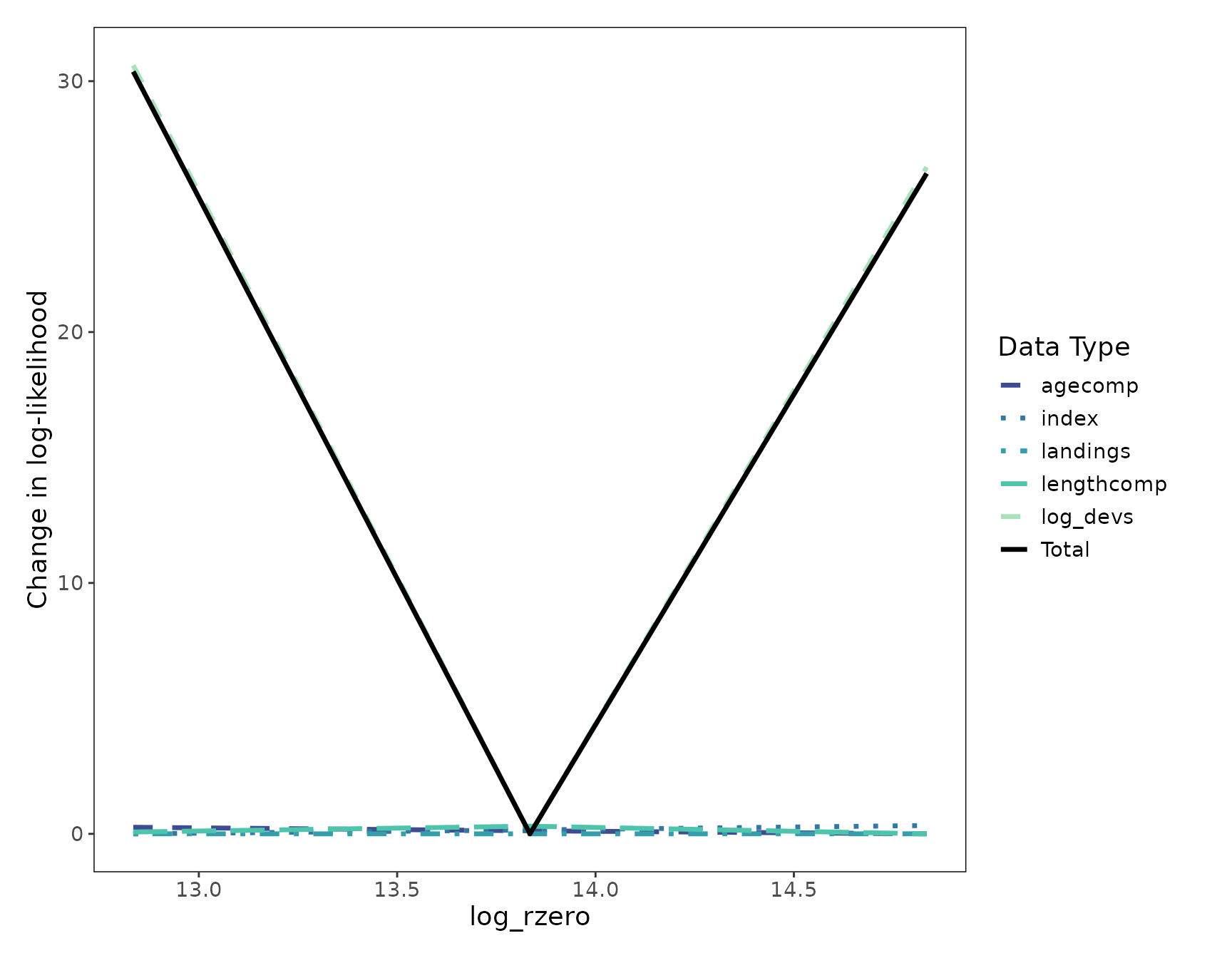

Curved lines showing change in likelihood in total and for each data type.

This function creates a ggplot object that can be customized and added onto. The default theme is stockplotr::theme_noaa, however to change the theme or colors used, you can simply add them after the main plot function.

fig_likelihood_custom_theme <- plot_likelihood(like_fit) +
  ggplot2::theme_bw()
print(fig_likelihood_custom_theme)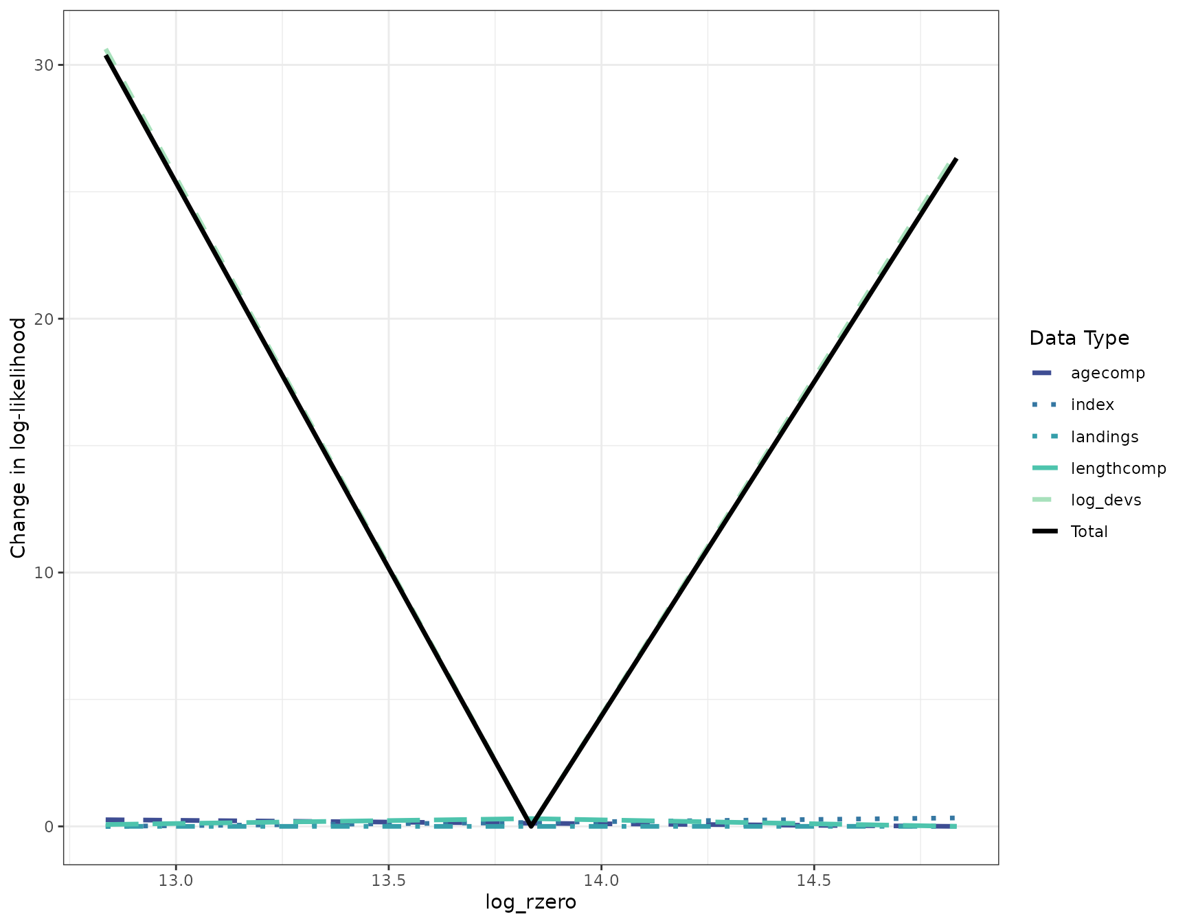

The same curved-line plot as above but with a different ggplot theme.

Clean up

Once you are finished running a FIMS model, it is always good practice to clear the C++ memory from one FIMS model run to the next.

clear()

Retrospective analysis

A retrospective analysis is a common model diagnostic used to assess the stability of estimates of parameters and derived quantities, such as fishing mortality and spawning biomass, and if there is a consistent pattern in the estimates as years of data are removed. The process involves removing n years of data from the end of the time series and refitting the model. This is an iterative process where the user typically runs 5–10 models, with each run (often called “peels”) progressively removing another year of data. Estimates from these peels are then compared to the model run with the full dataset (reference model). The Mohn’s rho statistic can be used to compare the relative difference between the reference model and each peel. Mohn’s rho statistic is calculated as:

$\rho = \frac{1}{n} \sum_{i=1}^{n} \frac{x_{p,y} - x_{base,y}}{x_{base,y}}$

where $n$ is the number of retrospective peels, $x_{p, y}$ is the estimated value (e.g., spawning biomass, fishing mortality, etc.) from peel $p$ at its terminal year $y$ , and $x_{base,y}$ is the value from the reference model, $base$ , at that same year $y$ .

Some things to note about run_fims_retrospective() is that you can provide data that is already a FIMSFrame object or you can give it one that is not. In the example below, we are using the FIMSFrame data object (data_4_model) created above. Additionally, it expects a vector of positive values of years_to_remove from the base model, starting from 0. If you are running many peels, it may be more efficient to use multiple cores, which can be specified with the n_cores argument.

NOTE: If left empty, the default for n_cores is one less than the number of cores on your machine so this could unexpectedly use up a lot of your computing power.

retro_fit <- run_fims_retrospective(
  years_to_remove = 0:2,
  data_4_model,
  parameters,
  n_cores = 1
)
#> ℹ ...Running sequentially on a single core
#> ℹ running model with 0 years of data removed
#> ✔ Starting optimization ...
#> ℹ Restarting optimizer 3 times to improve gradient.
#> ℹ Maximum gradient went from 0.00165 to 0.00031 after 3 steps.
#> ✔ Finished optimization
#> ✔ Finished sdreport
#> ℹ FIMS model version: 0.9.3.9000
#> ℹ Total run time was 1.44278 minutes
#> ℹ Number of parameters: fixed_effects=49, random_effects=29, and total=78
#> ℹ Maximum gradient= 0.00031
#> ℹ Negative log likelihood (NLL):
#> • Marginal NLL= 3231.28735
#> • Total NLL= 3164.86339
#> ℹ Terminal SB= 1728.68508
#> ℹ running model with 1 years of data removed
#> 
#> ✔ Starting optimization ...
#> ℹ Restarting optimizer 3 times to improve gradient.
#> ℹ Maximum gradient went from 0.00638 to 0.00025 after 3 steps.
#> ✔ Finished optimization
#> ✔ Finished sdreport
#> ℹ FIMS model version: 0.9.3.9000
#> ℹ Total run time was 1.49698 minutes
#> ℹ Number of parameters: fixed_effects=49, random_effects=29, and total=78
#> ℹ Maximum gradient= 0.00025
#> ℹ Negative log likelihood (NLL):
#> • Marginal NLL= 3132.00827
#> • Total NLL= 3066.98892
#> ℹ Terminal SB= 1654.148
#> ℹ running model with 2 years of data removed
#> 
#> ✔ Starting optimization ...
#> ℹ Restarting optimizer 3 times to improve gradient.
#> ℹ Maximum gradient went from 0.00164 to 0.00173 after 3 steps.
#> ✔ Finished optimization
#> ✔ Finished sdreport
#> ℹ FIMS model version: 0.9.3.9000
#> ℹ Total run time was 1.50064 minutes
#> ℹ Number of parameters: fixed_effects=49, random_effects=29, and total=78
#> ℹ Maximum gradient= 0.00173
#> ℹ Negative log likelihood (NLL):
#> • Marginal NLL= 3036.85438
#> • Total NLL= 2973.27387
#> ℹ Terminal SB= 1500.13192

Mohn’s Rho

Once you have run a retrospective, you can then calculate the Mohn’s rho statistic for spawning biomass by:

rho_sb <- calculate_mohns_rho(retro_fit, quantity = "spawning_biomass")

Visualize the results

To visualize the results of the retrospective analysis, we can use plot_retrospective() to display the quantity of interest. Below, we want to assess the impact on spawning biomass. The function returns a ggplot object, which you can customize by adding add layers as you normally would to a ggplot. For example, below, we specify the x and y axes labels and the legend title.

fig_retrospective_ssb <- stockplotr::plot_spawning_biomass(
  retro_fit$estimates |>
    dplyr::rename(
      year = year_i,
      estimate = estimated
    ) |>
    dplyr::mutate(
      uncertainty_label = "se"
    ),
  group = "retrospective_peel"
)
print(fig_retrospective_ssb)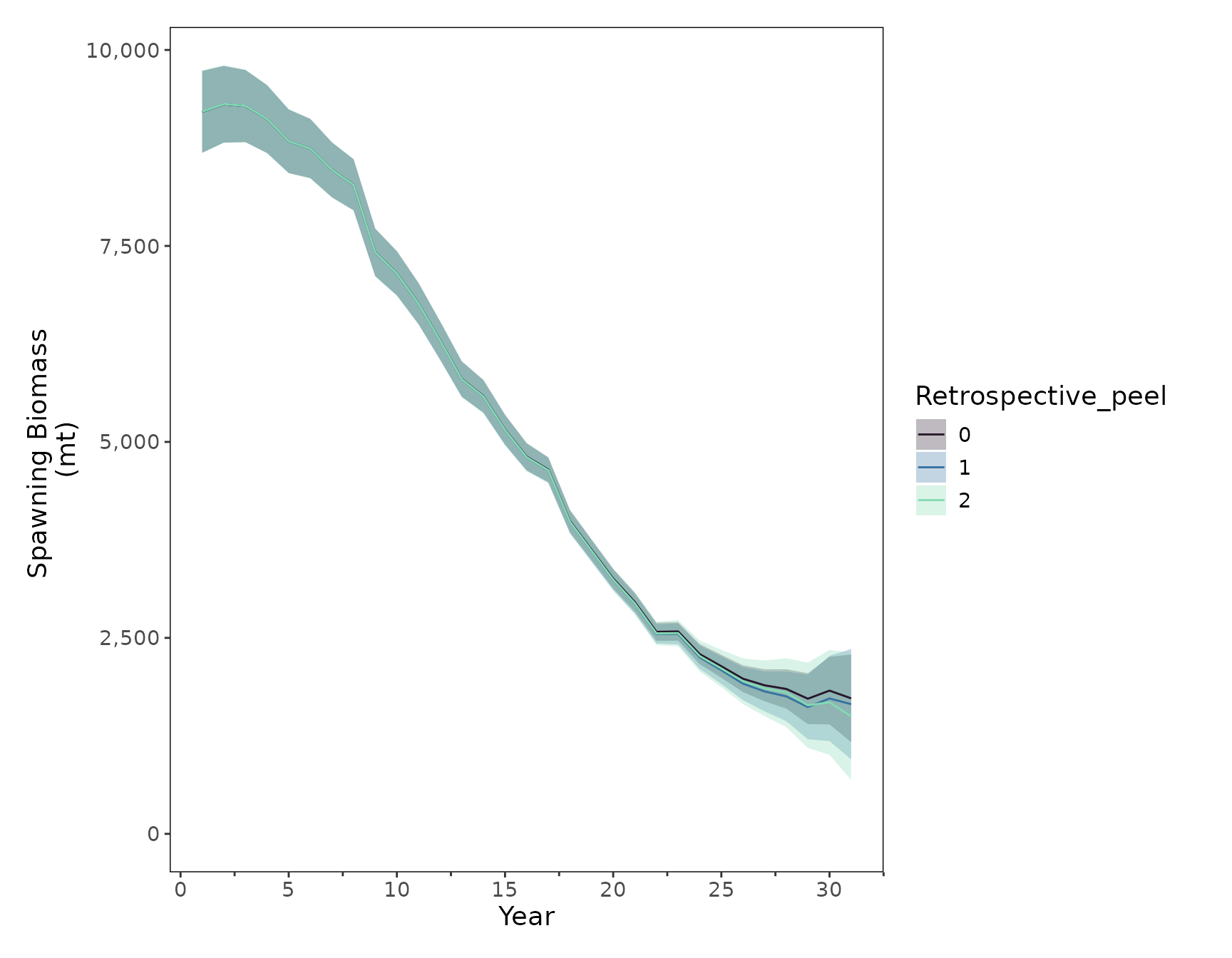

Plot of spawning biomass showing a small negative bias with removed years.

We can compare the spawning biomass estimates from the reference model and each peel for the last six years.

retro_fit[["estimates"]] |>
  dplyr::filter(label == "spawning_biomass") |>
  dplyr::select(label, year_i, estimated, retrospective_peel) |>
  tidyr::pivot_wider(
    names_from = retrospective_peel,
    values_from = estimated
  ) |>
  dplyr::rename(
    "Year" = year_i,
    "Reference model" = `0`,
    "Peel 1" = `1`,
    "Peel 2" = `2`
  ) |>
  tail()
#> # A tibble: 6 × 5
#>   label             Year `Reference model` `Peel 1` `Peel 2`
#>   <chr>            <int>             <dbl>    <dbl>    <dbl>
#> 1 spawning_biomass    26             1979.    1916.    1947.
#> 2 spawning_biomass    27             1895.    1817.    1856.
#> 3 spawning_biomass    28             1849.    1754.    1801.
#> 4 spawning_biomass    29             1724.    1618.    1640.
#> 5 spawning_biomass    30             1827.    1727.    1678.
#> 6 spawning_biomass    31             1729.    1654.    1500.

Clean up

Once you are finished running a FIMS model, it is always good practice to clear the C++ memory from one FIMS model run to the next.

clear()