convert_output_asap <- function(report, fleet_names) {
years <- seq(report$parms$styr, report$parms$endyr)
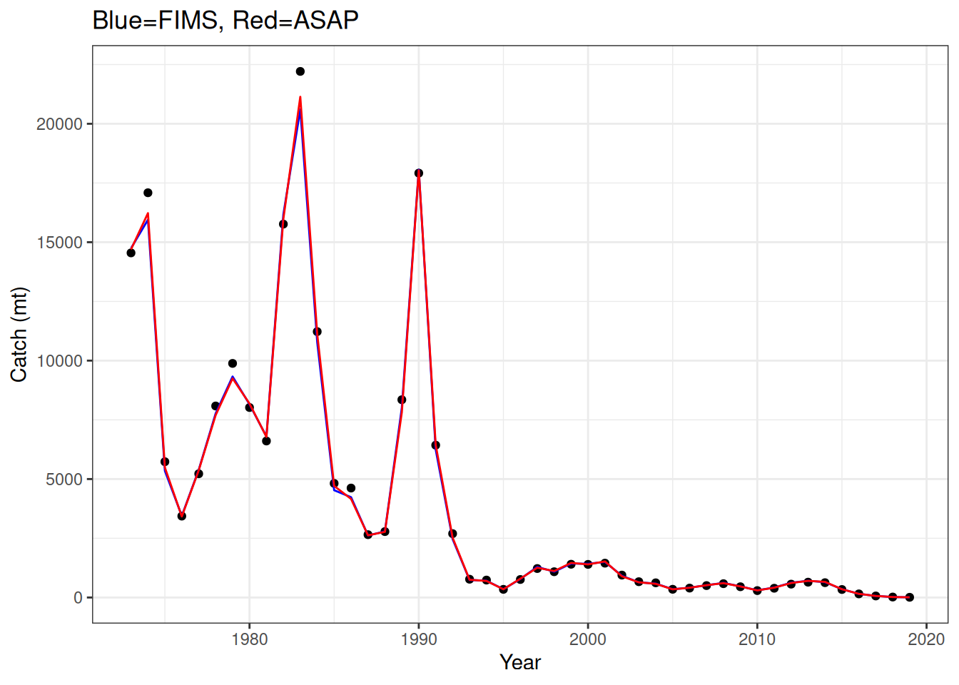
catch <- data.frame(
module_name = "Fleet",
module_id = rep(seq(NROW(report$catch.pred)), each = length(years)),
label = "landings_expected",
year_i = rep(seq(NCOL(report$catch.pred)), NROW(report$catch.pred)),
estimate = c(report$catch.pred),
estimation_type = "derived_quantity"
)
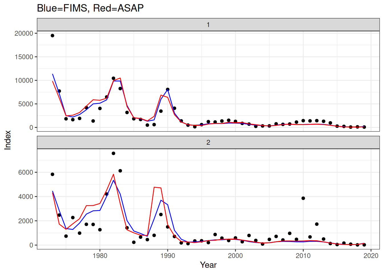
index <- data.frame(
module_name = "Fleet",
module_id = rep(seq(report$index.pred) + NROW(report$catch.pred), each = length(years)),
label = "indices_expected",
year_i = unlist(report$index.year.counter),
estimate = unlist(report$index.pred),
estimation_type = "derived_quantity"
)
index_observed <- index |>
dplyr::mutate(
label = "indices_observed",
estimate = unlist(report$index.obs)
)
spawning_biomass <- data.frame(
module_name = "Population",
label = "spawning_biomass",
year_i = seq(years),
estimate = report$SSB * 0.5,
estimation_type = "derived_quantity"
)
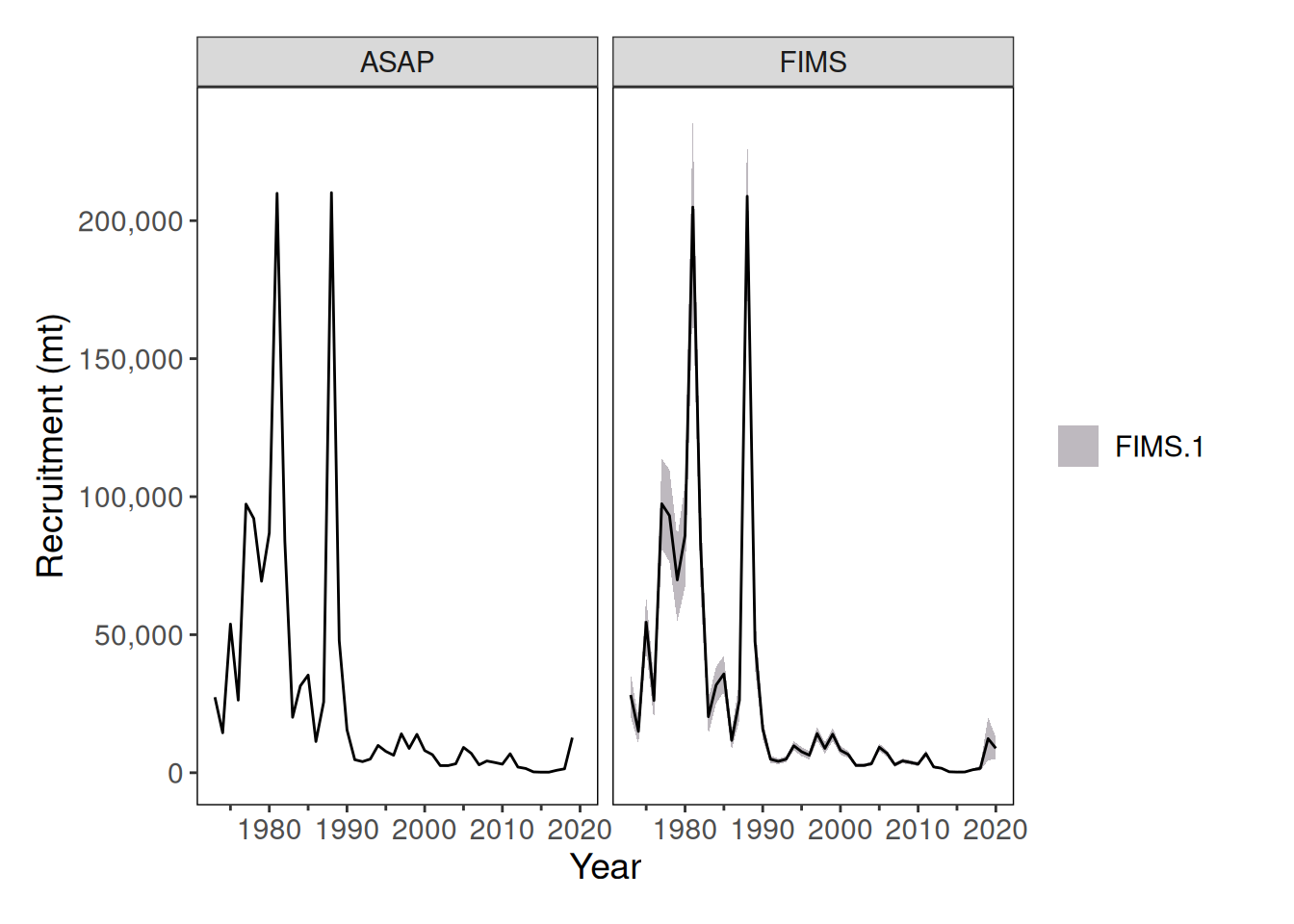
expected_recruitment <- data.frame(
module_name = "Population",
label = "expected_recruitment",
year_i = seq(years),
estimate = as.numeric(report$N.age[, 1]),
estimation_type = "derived_quantity"
)
# I don't know the structure of F.report when more than one fleet is present
log_Fmort <- data.frame(
module_name = "Fleet",
module_id = 1,
label = "log_Fmort",
type = "vector",
year_i = seq(years),
estimate = log(report$F.report),
estimation_type = "fixed_effects"
)
log_init_naa <- data.frame(
module_name = "Population",
label = "log_init_naa",
type = "vector",
age_i = rep(
seq(NCOL(report$N.age)),
NROW(report$N.age)
),
year_i = rep(
seq(NROW(report$N.age)),
each = NCOL(report$N.age)
),
estimate = log(c(t(report$N.age))),
estimation_type = "fixed_effects"
)
dplyr::bind_rows(
catch, index, index_observed,
spawning_biomass, expected_recruitment, log_Fmort, log_init_naa
) |>
dplyr::left_join(
data.frame(
year = years,
year_i = seq(years)
),
by = "year_i"
) |>
dplyr::mutate(
uncertainty = NA_real_,
uncertainty_label = "se",
fleet = as.character(factor(module_id, labels = fleet_names)),
era = "time"
)
}
output_asap <- convert_output_asap(rdat, get_fleets(data_4_model))
output_fims <- output |>
dplyr::mutate(
uncertainty_label = "se",
year = year_i + FIMS::get_start_year(data_4_model) - 1,
estimate = estimated,
era = "time"
)
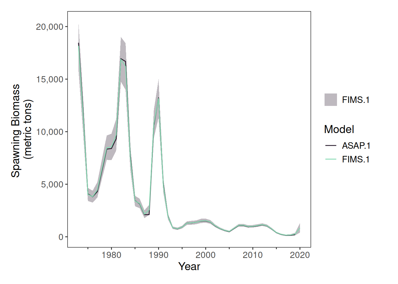
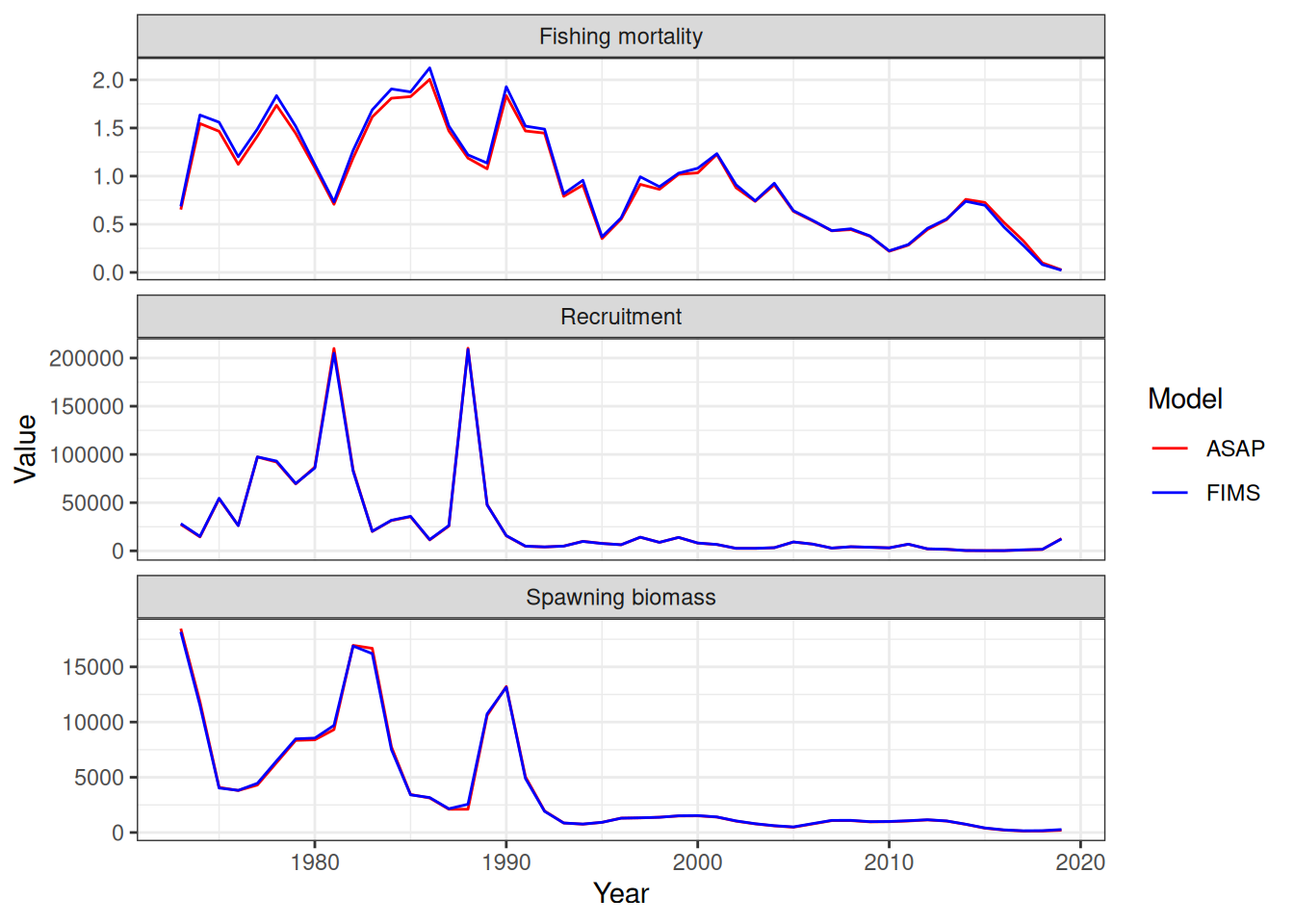
stockplotr::plot_spawning_biomass(
list(
"ASAP" = output_asap,
"FIMS" = output_fims
)
)