SWFSC Case Study Pacific sardine

The setup

Code

# Names of required packages
packages <- c("dplyr", "tidyr", "ggplot2", "TMB", "reshape2", "here", "remotes", "lubridate")

# Install packages not yet installed
installed_packages <- packages %in% rownames(installed.packages())
if (any(installed_packages == FALSE)) {
  install.packages(packages[!installed_packages], repos = "http://cran.us.r-project.org")
}

remotes::install_github("NOAA-FIMS/FIMS")
remotes::install_github("r4ss/r4ss")

# Load packages
invisible(lapply(packages, library, character.only = TRUE))

library(FIMS)

R_version <- version$version.string
TMB_version <- packageDescription("TMB")$Version
FIMS_commit <- substr(packageDescription("FIMS")$GithubSHA1, 1, 7)

source(file.path("R", "utils.R"))

Code

# R_version <- version$version.string
# TMB_version <- packageDescription("TMB")$Version
# FIMS_commit <- substr(packageDescription("FIMS")$GithubSHA1, 1, 7)

Add a chunk of code describing your setup

R version: R version 4.4.2 (2024-10-31)
TMB version: 1.9.16
FIMS commit: eca8095
Stock name: Pacific sardine northern subpopulation
Region: SWFSC
Analyst: Peter Kuriyama

Add a bulleted list and script describing simplifications you had to make

How I simplified my assessment * Convert two-semester time step to annual * Sum the catch values for MexCal S1 and S2 * Sum the age comps for MexCal S1 and S2 * Drop PNW fishing fleet data (catch and age comp data) * Drop spring AT survey index values * Use expected summary biomass values as AT survey CPUE * Fix Q=1 for AT survey, rather than have fixed, year-specific values * No SR_regime parameter estimated (population assumed to start a equilibrium) * Fixed M at 0.8 * Assume time-invariant logistic selectivity AT survey fleets (time-varying age-0 in benchmark assessment) * Assume time-invariant logistic selectivity MexCal fleet (time-varying in benchmark assessment) * Lorenzen age M -> one M value * No ageing error in FIMS? * Assume time-invariant weight at age for the fishery and survey

Add your script that sets up and runs the model

Code

# options(max.print = 1000, device = 'windows')
#
# library(plyr)
# library(reshape2)
# library(tidyverse)
# library(devtools)
# library(patchwork)
# library(scales)
# withr::local_options(pkg.build_extra_flags = FALSE)
#
# library(TMB)
# library(r4ss)
#
# #Local version of FIMS downloaded last week
# # devtools::load_all("../fims_v2/FIMS")
#
#
# # devtools::install_github("NOAA-FIMS/FIMS")
# # pak::pkg_install("NOAA-FIMS/FIMS")
#
# library(FIMS)

clear()
rm(list = ls())

#--------------------------------------------------------
#Logistic function for later use
logistic <- function(x, slope, inflection_point){
  out <- 1 / (1 + exp(-1 * slope * (x - inflection_point)))
  out <- data.frame(x = x, value = out)
  return(out)
}

#--------------------------------------------------------
#Manually enter data

# setwd("C://Users//peter.kuriyama//SynologyDrive/Research//noaa//FIMS")

#-----Catch
catch <- data.frame(year = 2005:2023, catch = c(29188.50, 53107.00, 69929.40,
                                                56317.80, 33546.40, 17466.40, 39383.10, 2585.38, 5705.77, 2558.63, 7.18, 428.26,
                                                347.11, 514.20, 619.04, 653.15, 285.89, 508.02, 152.31))

# ggplot(catch, aes(x = year, y = catch)) + geom_point() +
#   geom_line() + scale_y_continuous(label = comma)


fimscatch <- tibble::tibble(type = "landings", name = "fleet1",
                    age = NA, datestart = paste0(catch$year, "-01-01"),
                    dateend = paste0(catch$year, "-12-31"), value = catch$catch,
                    unit = "mt", uncertainty = 0.05)

#-----CPUE
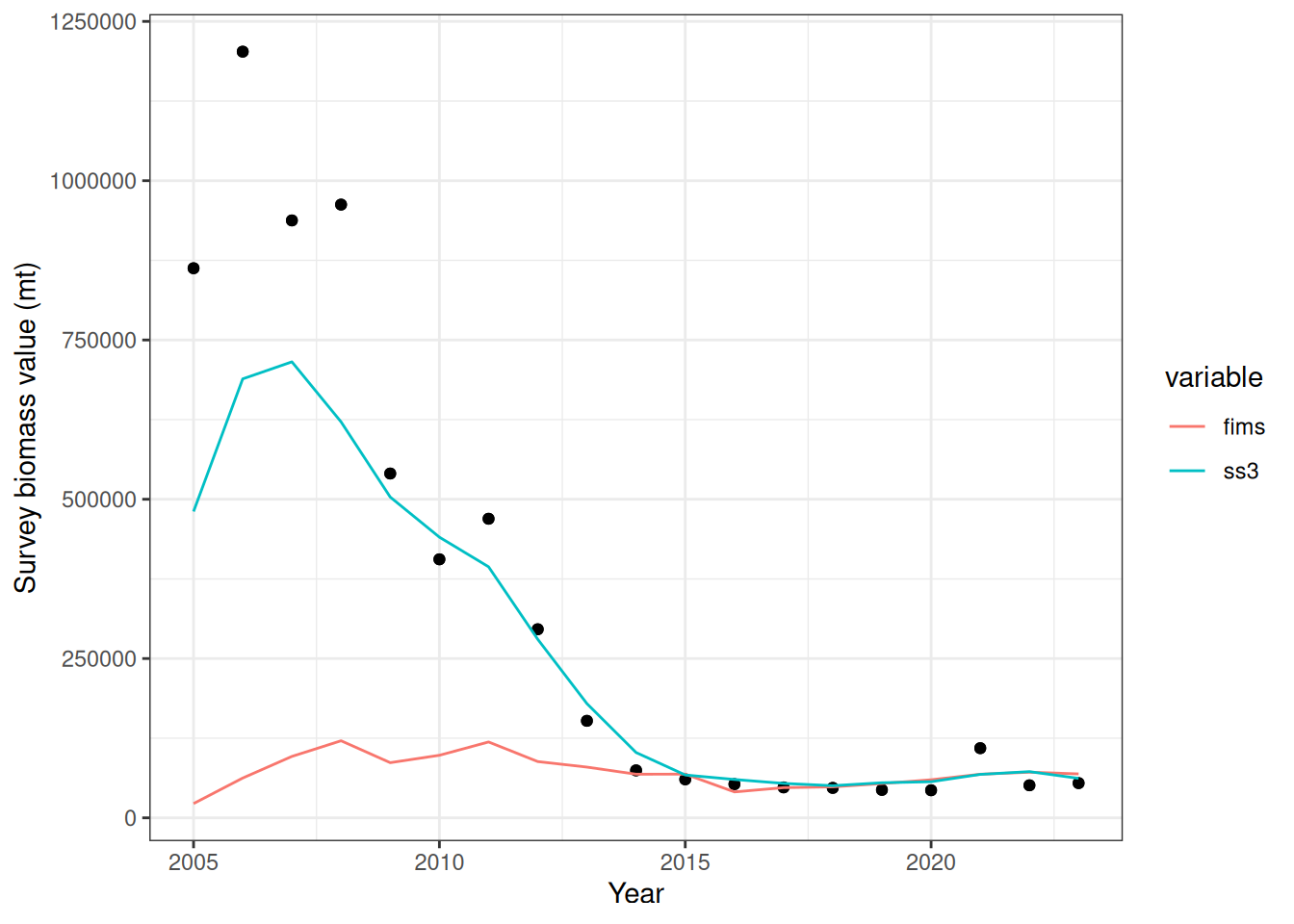
cpue <- data.frame(year = 2005:2023, obs = c(649619.0, 899635.0, 956354.0, 863281.0, 652029.0,
                                             504970.0, 395783.0, 293980.0, 182417.0, 89260.1,
                                             46403.0, 40704.0, 44592.1, 48789.1, 53551.8,
                                             59765.8, 68451.7, 71612.5, 68957.9))


# ggplot(cpue, aes(x = year, y = obs)) + geom_point() + geom_line() +
#   scale_y_continuous(label = comma)

fimsindex <- tibble::tibble(type = "index", name = "survey1",
                    age = NA, datestart = paste0(cpue$year, "-01-01"),
                    dateend = paste0(cpue$year, "-12-31"),
                    value = cpue$obs, unit = 'mt', uncertainty = .3)
fimsindex$unit <- ""

#-----Age compositions
acomps <- utils::read.csv("data_files/sardine_acomps.csv") |>
  dplyr::mutate(value_prop = value / Nsamp) # convert age-comp data to proportions, to match fims-demo.Rmd

fimsage <- tibble::tibble(type = "age", name = acomps$name,
                  age = acomps$age, datestart = paste0(acomps$Yr, "-01-01"),
                  dateend = paste0(acomps$Yr, "-12-31"),
                  value = acomps$value_prop, unit = "proportion", uncertainty = acomps$Nsamp)

# Fill in missing name/year rows with -999s for value and "" for uncertainty
  # This works the same as not doing anything, but is not necessary
# blank_age_grid <- expand.grid(name = c("fleet1", "survey1"),
#                               age = 0:8,
#                               yr = 2005:2023)
# blank_age <- tibble::tibble(type = "age", name = blank_age_grid$name,
#                     age = blank_age_grid$age,
#                     datestart = paste0(blank_age_grid$yr, "-01-01"),
#                     dateend = paste0(blank_age_grid$yr, "-12-31"),
#                     value = -999, unit = "proportion", uncertainty = NA)
# missing_ages <- blank_age |>
#   mutate(name_date = paste0(name, datestart)) |>
#   filter(!(name_date %in% paste0(fimsage_init$name, fimsage_init$datestart))) |>
#   select(-name_date)
# fimsage <- rbind(fimsage, missing_ages)

#fimsage$uncertainty <- 50 Leave as empirical values

fimscatch$value <- fimscatch$value
fimsindex$unit <- ""

#-----Weight-at-age
  # Q: What are the differences in how SS3 and FIMS process wtatage inputs/units?
  # A: SS3 assumes WAA is expressed in kg, and then converts to mt for biomass calculations
      # SS3 also expresses natage in terms of 1000s/fish
    # FIMS assumes WAA is expressed in mt, but expresses natage in fish
    # WAA input values are supplied to SS3 in kg and FIMS in mt
    # Model now correctly processes inputs and provides comparable NAA, WAA, and biomass outputs to SS3
wtatage <- r4ss::SS_readwtatage("data_files/sardine_wtatage.ss_new") |>
  dplyr::filter(fleet %in% c(1, 2)) |>
  dplyr::mutate(fleet = ifelse(fleet == 1, "fleet1", "survey1")) |>
  tidyr::pivot_longer(cols = `0`:`10`, names_to = "age", values_to = "value") |>
  dplyr::filter(year != 2024, !(age %in% c("9", "10"))) |> # Trim ages 9 and 10 to match age-comps
  dplyr::mutate(value = value / 1000) # WAA converted from kg to mt
fimswaa <- tibble::tibble(
  type = "weight-at-age",
  name = wtatage$fleet,
  age = wtatage$age,
  datestart = paste0(wtatage$year, "-01-01"),
  dateend = paste0(wtatage$year, "-12-31"),
  value = wtatage$value,
  unit = "mt",
  uncertainty = NA
)

#Combine everything, format
fimsdat <- rbind(fimscatch, fimsindex, fimsage, fimswaa)
fimsdat$age <- as.integer(fimsdat$age)
fimsdat$value <- as.numeric(fimsdat$value)

# Convert to FIMSFrame
final_fimsdat <- FIMSFrame(fimsdat)

# Define fleet specifications for fleet1 and survey1
fleet1 <- survey1 <- list(
  selectivity = list(form = "LogisticSelectivity"),
  data_distribution = c(
    Index = "DlnormDistribution",
    AgeComp = "DmultinomDistribution",
    LengthComp = "DmultinomDistribution"
  )
)

# Create default recruitment, growth, and maturity parameters
default_parameters <- final_fimsdat |>
  create_default_parameters(
    fleets = list(fleet1 = fleet1, survey1 = survey1)
  )

# Update parameters
  # Control how parameters are updated
estimate_fish_selex <- FALSE
estimate_survey_selex <- FALSE
estimate_q <- FALSE #Fix at 1
estimate_F <- TRUE
estimate_recdevs <- TRUE
estimate_init_naa <- TRUE
estimate_log_rzero <- TRUE
steep <- 0.6 # sardine steepness is fixed at 0.6
M_value <- 0.8 #.8 worked pretty well
rzero <- 17 #14.2 is log(R0) in sardine simplified model
nyears <- get_n_years(final_fimsdat)
years <- get_start_year(final_fimsdat):get_end_year(final_fimsdat)
nages <- get_n_ages(final_fimsdat)
ages <- get_ages(final_fimsdat)
init_naa <- exp(rzero) * exp(-(ages - 1) * M_value)
init_naa[nages] <- init_naa[nages] / M_value # sum of infinite series

  # Update parameters
parameters <- default_parameters |>
  update_parameters( # update fleet1 specifications
    modified_parameters = list(
      fleet1 = list(
        LogisticSelectivity.inflection_point.value = 1,
        LogisticSelectivity.inflection_point.estimated = estimate_fish_selex,
        LogisticSelectivity.slope.value = 5,
        LogisticSelectivity.slope.estimated = estimate_fish_selex,
        Fleet.log_Fmort.value = log(rep(0.2, nyears)),
        Fleet.log_Fmort.estimated = estimate_F,
        DlnormDistribution.log_sd.value = rep(log(sqrt(log(0.01^2 + 1))), nyears)
      )
    )
  ) |>
  update_parameters( # update survey1 specifications
    modified_parameters = list(
      survey1 = list(
        LogisticSelectivity.inflection_point.value = 1.2,
        LogisticSelectivity.inflection_point.estimated = estimate_survey_selex,
        LogisticSelectivity.slope.value = 2,
        LogisticSelectivity.slope.estimated = estimate_survey_selex,
        Fleet.log_q.value = 0,
        Fleet.log_q.estimated = estimate_q,
        DlnormDistribution.log_sd.value = rep(log(sqrt(log(0.1^2 + 1))), nyears)
      )
    )
  ) |>
  update_parameters(
    modified_parameters = list(
      recruitment = list(
        BevertonHoltRecruitment.log_rzero.value = rzero,
        BevertonHoltRecruitment.log_rzero.estimated = estimate_log_rzero,
        BevertonHoltRecruitment.logit_steep.value = -log(1.0 - steep) + log(steep - 0.2),
        BevertonHoltRecruitment.log_devs.value = rep(log(1), nyears-1),
        DnormDistribution.log_sd.value = log(1.2)
      )
    )
  ) |>
  update_parameters(
    modified_parameters = list(
      maturity = list(
        LogisticMaturity.inflection_point.value = 1.2,
        LogisticMaturity.inflection_point.estimated = FALSE,
        LogisticMaturity.slope.value = 1.5, # arbitrary guess
        LogisticMaturity.slope.estimated = FALSE
      )
    )
  ) |>
  update_parameters(
    modified_parameters = list(
      population = list(
        Population.log_M.value = rep(log(M_value), nages * nyears),
        Population.log_init_naa.value = log(init_naa),
        Population.log_init_naa.estimated = estimate_init_naa
      )
    )
  )

# Fit the model
fit <- parameters |>
  initialize_fims(data = final_fimsdat) |>
  fit_fims(optimize = TRUE)

✔ Starting optimization ...
ℹ Restarting optimizer 3 times to improve gradient.
ℹ Maximum gradient went from 0.00769 to 0.00016 after 3 steps.
✔ Finished optimization
✔ Finished sdreport
ℹ FIMS model version: 0.3.0.1
ℹ Total run time was 0.10608 seconds
ℹ Number of parameters: total=47, fixed_effects=47, and random_effects=0
ℹ Maximum gradient= 0.00016
ℹ Negative log likelihood (NLL):
• Marginal NLL= 1044.96182
• Total NLL= 1044.96182
ℹ Terminal SB=

Code

# Get information about the model and print a few characters to the screen
recruitment_log <- get_log_module("information")
substr(recruitment_log, 1, 100)

[1] "[\n{\n\"timestamp\" : \"Mon Feb 17 14:59:48 2025\",\n\"level\" : \"info\",\n\"message\" : \"Initializing fleet 1\",\n"

Code

# Clear memory post-run
clear()

Add your comparison figures

Code

load("data_files/sardine_simplified_res.Rdata")

#------------------------------------------------------------------------
#------SSB
# Q: Is 'ssb' from  get_report(fit) calculated assuming 2 genders and a 50:50 ratio?
  # If so, it might explain the discrepancy between ss3 (1 gender model) and fims (2 genders)
ssbs <- ssres$timeseries |>
  dplyr::select(Yr, SpawnBio) |>
  dplyr::mutate(fims = c(0, 0, get_report(fit)[["ssb"]][[1]]))
names(ssbs)[2] <- 'ss3'

ssbs |>
  dplyr::filter(Yr >= 2005, Yr < 2024) |>
  tidyr::pivot_longer(names_to = "variable", cols = dplyr::matches("ss3|fims")) |>
  ggplot2::ggplot(ggplot2::aes(x = Yr, y = value, group = variable, color = variable)) +
  ggplot2::geom_point() +
  ggplot2::geom_line() +
  ggplot2::ylab("Spawning biomass (mt)") +
  ggplot2::theme_bw() +
  ggplot2::xlab("year") +
  ggplot2::theme(legend.position.inside = c(.9, .9))

Code

ggplot2::ggsave(
  "figures/SWFSC-sardine-sb.png",
  width = 7.35,
  height = 4.8
)

#------------------------------------------------------------------------
#------Index fits
index <- ssres$cpue |>
  dplyr::select(Yr, Obs, Exp)
names(index) <- c("year", 'obs', 'ss3')
index$fims <- get_report(fit)[["exp_index"]][[2]]
index |>
  tidyr::pivot_longer(names_to = "variable", cols = dplyr::matches("ss3|fims")) |>
  ggplot2::ggplot(ggplot2::aes(x = year)) +
  ggplot2::geom_point(ggplot2::aes(y = obs)) +
  ggplot2::geom_line(ggplot2::aes(y = value, color = variable, group = variable)) +
  ggplot2::theme_bw() +
  ggplot2::theme(legend.position.inside = c(.9, .9)) +
  ggplot2::xlab("Year") +
  ggplot2::ylab("Survey biomass value (mt)")

Code

ggplot2::ggsave("figures/SWFSC-sardine-surveyfit.png", width = 6.8, height = 5.25)

#------------------------------------------------------------------------
#-----Calculate age-1+ biomass
#Multiply numbers at age by weight at age and sum
naa <- get_report(fit)[["naa"]][[1]]

naa1 <- tidyr::crossing(c(years, 2024), ages) |>
  dplyr::mutate(naa = naa) |>
  as.data.frame()
names(naa1) <- c("year", 'age', 'value')
naa1$cohort <- naa1$year - naa1$age

#Format Weight at age (identical WAA for each year and fleet)
waa <- data.frame(
  age = wtatage$age[(wtatage$year == 2005 & wtatage$fleet == "fleet1")],
  waa = wtatage$value[(wtatage$year == 2005 & wtatage$fleet == "fleet1")]
) |>
  dplyr::mutate(age = as.integer(age))

naa1 <- naa1 |>
  dplyr::left_join(waa, by = "age")


naa1 <- naa1 |>
  dplyr::mutate(weight = value * waa)
age1plus <- naa1 |>
  dplyr::filter(age != 0) |>
  dplyr::group_by(year) |>
  dplyr::summarize(summbio = sum(weight))

bio1 <- ssres$timeseries |>
  dplyr::filter(Seas == 1) |>
  dplyr::select(Yr, Bio_smry) |>
  dplyr::mutate(year = Yr, ss3bio = Bio_smry) |>
  dplyr::select(-Yr, -Bio_smry)


age1plus <- age1plus |>
  dplyr::left_join(bio1, by = "year")

names(age1plus) <- c("year", "fims", "ss3")

#Full time series of age-1+ biomass
age1plus |>
  reshape2::melt(id.var = "year") |>
  ggplot2::ggplot(ggplot2::aes(x = year, y = value, group = variable, color = variable)) +
  ggplot2::geom_point() +
  ggplot2::geom_line() +
  ggplot2::ylab("Age-1+ biomass (mt)") +
  ggplot2::theme_bw() +
  ggplot2::theme(legend.position.inside = c(.9, .9))

Code

ggplot2::ggsave("figures/SWFSC-sardine-age1plusbio.png", width = 6.8, height = 5.25)

#Zoomed in time series of age-1+
age1plus |>
  reshape2::melt(id.var = "year") |>
  dplyr::filter(year >= 2010) |>
  ggplot2::ggplot(ggplot2::aes(x = year, y = value, group = variable, color = variable)) +
  ggplot2::geom_point() +
  ggplot2::geom_line() +
  ggplot2::theme_bw() +
  ggplot2::ylab("Age-1+ biomass (mt)") +
  ggplot2::theme(legend.position.inside = c(.9, .9))

Code

ggplot2::ggsave(
  "figures/SWFSC-sardine-age1plusbio_zoomedin.png",
  width = 6.8,
  height = 5.25
)


#------------------------------------------------------------------------
#------Recruitment
# Divide FIMS recruits by 1000 to match reporting in SS3
recs <- ssres$timeseries |>
  dplyr::select(Yr, Recruit_0) |>
  dplyr::mutate(fims = c(0, 0, get_report(fit)[["recruitment"]][[1]]) / 1000)
names(recs)[2] <- "ss3"

recs |>
  dplyr::filter(Yr >= 2005, Yr < 2024) |>
  reshape2::melt(id.var = "Yr") |>
  ggplot2::ggplot(ggplot2::aes(x = Yr, y = value, group = variable, color = variable)) +
  ggplot2::theme_bw() +
  ggplot2::geom_point() +
  ggplot2::geom_line() +
  ggplot2::theme(legend.position.inside = c(.9, .9)) +
  ggplot2::ylab("Recruits (x1000)")

Code

ggplot2::ggsave("figures/SWFSC-sardine-recruitment.png", width = 6.8, height = 5.25)


#------------------------------------------------------------------------
#------Fixed selectivities
#Are fixed but plot for comparison's sake
##Fishery

sel_fishery <- logistic(ages,
                        slope = parameters$parameters$fleet1$LogisticSelectivity.slope.value,
                        inflection_point = parameters$parameters$fleet1$LogisticSelectivity.inflection_point.value)

names(sel_fishery) <- c("age", "fims")

sel_fishery$ss3 <- ssres$ageselex |>
  dplyr::filter(Yr == 2005, Factor == "Asel", Fleet == 1) |>
  dplyr::select(as.character(0:8)) |>
  t()
sel_fishery <- sel_fishery |>
  reshape2::melt(id.var = "age")

Warning: attributes are not identical across measure variables; they will be
dropped

Code

ggplot2::ggplot(
  sel_fishery,
  ggplot2::aes(x = age, y = value, group = variable, color = variable)
) +
  ggplot2::geom_point() +
  ggplot2::geom_line()

Code

#-----------Survey
sel_survey <- logistic(ages,
                       slope = parameters$parameters$survey1$LogisticSelectivity.slope.value,
                       inflection_point = parameters$parameters$survey1$LogisticSelectivity.inflection_point.value)

names(sel_survey) <- c("age", 'fims')

sel_survey$ss3 <- ssres$ageselex |>
  dplyr::filter(Yr == 2005, Factor == "Asel", Fleet == 2) |>
  dplyr::select(as.character(0:8)) |>
  t()
sel_survey <- sel_survey |>
  reshape2::melt(id.var = "age")

Warning: attributes are not identical across measure variables; they will be
dropped

Code

ggplot2::ggplot(
  sel_survey,
  ggplot2::aes(x = age, y = value, group = variable, color = variable)
) +
  ggplot2::geom_point() +
  ggplot2::geom_line()

Add comparison tables

What was your experience using FIMS? What could we do to improve usability?

Tools to check: * data were inputted correctly (dimension checks) * starting values and settings are reasonable * Perhaps have a model template file that will work as is, then users can modify as necessary * I had issues installing FIMS with install_github that seemed to be related to R settings

Model: * streamline configuration of fleets and maybe make it easier to add additional fleets (perhaps clone existing ones then change specific settings) * Think about ways to modify single model settings based on say different starting values

Output: * include all parameter values and names (fixed and estimated, also show starting values) * Code to generate a default set of figures and tables for use in assessment documents/presentations

List any issues that you ran into or found

Please open an issue if you found something new.

What features are most important to add based on this case study?

The ability to start the model at non-equilibrium conditions (In SS3 there is a SR_regime parameter and Initial F to match equilbirium age comps to first year of data age comps) *Does the model year start in the first year of the data input?

Add your pages to the project

Add the files to _quarto.yml